To obtain long-term geological records over millions of years we need to analyze something that persists for long time periods: rocks. What we will discuss is how we can use the limestone (mineral: calcite) of fossils in order to look at the temperature of sea water as well as at the volumes of the polar ice caps.

Oxygen isotopes in paleoceanography

Harold Urey first outlined the idea to use the oxygen isotopic composition of carbonates to deduce the temperature at which the carbonate was deposited (1948, Oxygen isotopes in nature and the laboratory, Science, v. 108, p. 489-496). These measurements are now one of the cornerstones of paleoceanographic research, but not always dominantly for derivation of paleotemperatures: the data are commonly used for evaluation of polar ice volume. Carbon isotopic data are obtained at the same time as oxygen isotopic data; we will come to carbon isotope data next week.

Oxygen isotope mass spectrometry (and some information on carbon)

The element oxygen occurs as 3 stable isotopes as explained in last week's handout: the common isotope ¹⁶O (99.765%), the rare isotope ¹⁸O (0.1995%), and the very rare isotope ¹⁷O (0.0355%). We just pay no attention to ¹⁷O because it is so very rare. An element must be in the gas phase if we want to measure its isotopic ratios in a mass-spectrometer, and the gas used for analysis of oxygen isotopes is CO₂. The element carbon occurs in two stable isotopes (in addition to the radioactive isotope ¹⁴C): the common isotope ¹²C (98.89%), and the rare isotope ¹³C (1.11%). CO₂ is liberated from CaCO₃ by dissolution in phosphoric acid (H₃PO₄):

3CaCO₃ + 2H₃PO₄ -> 3CO₂ + 3H₂O + Ca₃(PO₄)₂.

You do not have to know this equation, but notice that it is very important to adhere to strictly normalized reaction conditions, because only 2 of the 3 O-atoms in CaCO₃ are present in the CO₂-gas, and the third one moves into a water molecule, with the hydrogen from the acid. If conditions are not normalized, isotopic fractionation during dissolution will vary from sample to sample and all our data will just show that one day it was warmer in the lab than another day, or something else that we are not interested in.

A CO₂ molecule can thus have different molecular weights (the parameter measured in a mass-spectrometer) as a result of the presence of one of the three stable isotopes of oxygen and one of the two of carbon isotopes. The most common configurations of CO₂ are: ¹²C¹⁶O¹⁶O with a molecular weight 44, by far the most common molecule; ¹³C¹⁶O¹⁶O with a molecular weight 45, and ¹²C¹⁸O¹⁶O with molecular weight 46. These three molecules have no or only one of the rare isotopes. Molecules in which two rare isotopes are present are extremely rare, because the probability of pairing (for instance) two ¹⁸O-atoms in one CO₂ molecule by randomly moving atoms is infinitesimally small.

Isotope fractionation

Isotope fractionation is the partial separation of isotopes of the same element during physical (e.g., evaporation) or chemical (e.g., precipitation reaction) processes. The separation results from the small differences in physico-chemical properties of molecules containing different isotopes. Kinetic isotopic fractionation occurs when the rates of processes differ between isotopic species (as a result of molecules with the lighter isotope moving faster). Equilibrium isotope fractionation occurs as a result of differences in thermodynamic properties of molecules containing different isotopes:

Reaction 1: Ca²⁺ + 2HCO₃^- -> CaCO₃ + H₂O + CO₂, and

Reaction 2: H₂O + CO₂ -> 2HCO₃^- .

The first reaction says that calcium and bicarbonate ions (HCO₃^- ) dissolved in sea water react to form calcium carbonate (limestone), with water and carbon dioxide. Notice that reaction 2 shows that the carbon dioxide and water react together to form more bicarbonate.

The oxygen in bicarbonate, which is the most common carbon-bearing ion in the oceans, equilibrates isotopically with the oxygen in water in the oceans, and the bicarbonate is then used by organisms building carbonate shells. Isotope fractionation between two substances (such as the bicarbonate ion dissolved in water and carbonate) accompanying a specific process (such as the precipitation of calcite) is expressed in the fractionation factor (a):

a _(c-w) = R_c/R_w,

in which a _(c-w) is the fractionation factor , and Rc and Rw are the isotopic ratios (¹⁸O/¹⁶O) in calcite and in water, respectively. Note that the abundance of the rare isotope is divided by the abundance of the common isotope, so that R << 1. There is an inverse relation between the fractionation factor a and temperature, so that fractionation is less at higher temperatures, and a becomes equal to 1 (no fractionation) at very high temperatures. According to the equation derived from a study of experimental inorganic precipitation of calcite over a temperature range between 0 and 500^oC:

10³lna = 2.78 (T^-2.10⁶) -3.39,

where T is the temperature in degrees Kelvin.

Conventions in describing oxygen and carbon isotopes

The absolute abundance of an isotope is difficult to measure with sufficient accuracy, and therefore we compare isotopic ratios in a sample with those in a standard (as we do for ice samples), resulting in the delta-notation:

where d_(x) is the delta-value of a sample, and Rx and Rst are the isotopic ratios in sample and standard, respectively. The d-value is the relative difference in the isotopic ratio of the sample and the standard, expressed in part per mille (‰); that's why the right-hand side of the equation is multiplied by 10³ (1000). Carbon and oxygen data from carbonates are usually referred to the PDB standard (a belemnite, Belemnitella americana, from the Late Cretaceous PeeDee Formation in South Carolina). Oxygen isotopic compositions of water samples are referred to standard mean ocean water (SMOW). The scales are related to each other as follows:

d¹⁸O_{calcite (vs. SMOW)} = 1.03086 d¹⁸O_{calcite (vs. PDB)} + 30.86.

Oxygen isotopes in carbonates as paleo-thermometer

We can use the isotopic composition of a carbonate to deduce the temperature at which the calcite was precipitated. The empirically determined temperature equation (again - found by measuring the values in many samples) that is used most often in work with deep-sea carbonates is:

t^oC = 16.9 - 4.38 (d_c -d_w) + 0.1 (d_c -d_w) ²,

in which t^oC is the temperature in degrees Celsius, d_c is the oxygen isotopic composition of calcite, d_w the oxygen isotopic composition of the water from which it was precipitated. We measure d_c in order to derive t ^oC. At constant d_w, a temperature change of 4^oC corresponds to a change in d_c of about 1‰.

NOTE: pay attention: this reaction means that in carbonate heavier oxygen isotopes mean lower temperature, just the opposite of the situation for ice cores!!

We can use this method to find the temperature at which the calcite was precipitated only IF we know the isotopic composition of the water from which the calcite was precipitated. In addition, calcite in nature is not precipitated from water simply by a chemical reaction: the chemical reaction occurs within the bodies of organisms. For much paleoceanographic work various species of planktonic (floating in the water column) and benthic (living on the sea floor) foraminifera (unicellular organisms with a calcite shell) are used; the combination of data on planktonic and benthic species allows determination of temperatures in surface and deep waters.

Measurements on recent foraminifera have shown that many planktonic foraminifera precipitate their test fairly close to oxygen isotopic equilibrium, with fixed offsets within a species. One tries to analyzes mono-specific samples, so that the same offset from equilibrium applies to all samples. Planktonic foraminifera have short species-lives, and we have to analyze many different species if we want to obtain a long record; we do not know whether extinct species precipitated their test in equilibrium. We have some ways of testing this. Presently, different planktonic species live at different depths (thus at different temperatures) in the water column. Isotopic signals of different species within one sample differ, according to their depth-ranking, with the deepest-dwelling species having the highest d-values (lowest temperatures). We thus expect the planktonic species from any one sample to have a range of isotopic values, and the benthic foraminifera in the same sample should have even heavier values (colder water). Benthic foraminifera differ by species as to precipitation of calcite: some (e.g., Uvigerina) are close to equilibrium for oxygen, whereas others (e.g., Cibicidoides) have an offset, usually a fixed offset for a species or a genus (the so-called "vital effect", for Cibicidoides -0.64‰). These offsets can be calculated by studies of different recent species; deep-sea benthic taxa have very long morphospecies lives and thus we can use the same taxon for long intervals of earth history.

The oxygen isotopic composition of sea water.

It is one of the major problems in isotope paleoceanography that an estimate of the average isotopic composition of sea water (the d_w mentioned above) is necessary in order to estimate paleo-temperatures. For instance, the strongly negative isotopic ratios measured in well-preserved Paleozoic carbonates suggest that ocean temperatures at that time were over 50^oC, which may be unrealistic biologically, or that the overall isotopic composition of sea water was lighter. A change in isotopic composition of sea water over geologic time might have resulted from addition of juvenile water (from the Earth's mantle) with an isotopic signature of +7 to +9‰ at mid-oceanic ridges. Hydrothermal alteration of basalts at high temperatures increases the d¹⁸O of seawater even more. Studies of ophiolites (fossil mid ocean ridge basalts) in Oman, however, indicate that weathering of basalts at low temperatures, i.e., in contact with sea water, increases the d¹⁸O in the basalt, but decreases d¹⁸O in the circulating sea water. Thus the effect of basaltic weathering at low temperatures on the sea floor counteracts the effect of juvenile water input and hydrothermal alteration, with the most recent reports suggesting that the two processes are about in equilibrium. Low-temperature weathering of fresh, crystalline rocks on land also tends to make the isotopic composition of run-off, thus ultimately of sea water, lighter. Therefore it is a possibility that changes in the relative rates of spreading at oceanic ridges and weathering on land might cause changes in the long-term isotopic composition of the oceans. Such changes occur slowly (range: 10⁶ years), and thus the isotopic changes as a result of such processes must be slow.

The largest known, and fastest, effect on isotopic composition of the oceans in the Cenozoic (the last 65 million years) has been by the volume of the polar ice sheets. These ice sheets are strongly enriched in the LIGHT isotope of oxygen.This enrichment in light isotopes is a result of the evaporation of water dominantly at low latitudes, and long travel from tropics to poles of water vapor from which more and more relatively heavy water rains out.

Most water on Earth (97.25%) is stored in the oceans, 2.05% in ice (90% of which resides in the Antarctic ice sheet), with the remainder stored as ground water (0.68%), while the water occurring as freshwater (lakes and rivers), as soil moisture, in the biosphere and atmosphere is an insignificant amount. Oxygen isotopic fractionation occurs during evaporation and condensation of water, with enrichment of the heavier isotope in the liquid phase (a = 1.010 at 20^oC). Water vapor is thus isotopically light compared with the ocean water from which it evaporated, and condensed rain is isotopically heavy compared with the water vapor from which it condensed. Rain that falls inland is therefore more depleted in ¹⁸O than rain in coastal areas, because much rain condenses in coastal areas (especially when humid air has to move up to cross mountains), and the remaining water vapor traveling inland has been isotopically depleted.

With much simplification, we can say that in the subtropics evaporation strongly exceeds precipitation, and at temperate to high latitudes the reverse is true (more precipitation than evaporation). Thus there is a net transport of water vapor from subtropical to high latitudes, causing considerable heat-transport: the subtropics lose the heat of evaporation of water, the higher latitudes gain the heat of condensation. This is called latent heat transport. Water vapor generated in the subtropics is isotopically lighter than the sea-water from which it formed; rain falling out is heavier than the remaining vapor - which thus is depleted even more in the heavy isotope. We can see the Earth as an approximation of a multiple-stage distillation column, with reflux of the condensate to the reservoir; such a process is called Rayleigh-fractionation. The reservoir is the ocean, rain at different latitudes is the condensate at different stages, and the polar ice (which forms from the snow, formed from vapor that has traveled furthest away from the area of original evaporation) is the highest stage of the column (and is thus the most depleted in the heavy isotope).

The snow in the interior of Antarctica (a continent at high latitudes) is thus the most depleted precipitation on earth, with values as low as -60‰; in Antarctic coastal areas values are approximately between -17 and -30‰. The average isotopic composition of the Antarctic ice sheet with a volume of about 26 x 106 km3 is not known precisely (the ice sheet is up to 4 km thick), and must be estimated. Probably there is a larger contribution from the more depleted snow inland (the snow falling in the coastal areas changes into ice that is quickly calved off as bergs); estimates are on the order of -35 to -50‰. This means, of course, that the present ice sheets are strongly depleted in 18O as compared to ocean water, with an average d18O of -0.28‰. Present estimates indicate that the oxygen isotopic composition of the ocean as a whole would be about -1.26‰ if all the ice sheets melted. At the same time, the oceans become more saline in the presence of ice sheets; at the present average isotopic composition of ice sheets a melting of ice volume equivalent to a global rise in sea level of 10m would result in an ocean about 0.1‰ lighter isotopically, and 0.2‰ less saline.

In order to use oxygen isotopic data from carbonates to calculate paleo-temperatures, we thus have to make estimates of the volume of polar ice (e.g., using data on sea-level), and of its isotopic composition. The present Antarctic ice is extremely depleted in ¹⁸O partially because it the ice sheet is so large and the temperatures are so low; if the ice sheet was much smaller, its average isotopic composition would probably also be less depleted.

So what are the problems?

Oxygen isotope measurements give information on more than one aspect of the history of aoxygen isotopes in sea water:

• Temperature of water
• Volume of polar ice caps.

The snow in the interior of Antarctica (a continent at high latitudes) is the most depleted precipitation on earth, with values as low as -60‰. In Antarctic coastal areas values are between -17 and -30‰. The average isotopic composition of the Antarctic ice sheet with a volume of about 26 million km³ is not known precisely (the ice sheet is up to 4 km thick), and must be estimated. Probably there is a larger contribution from the more depleted snow inland (the snow falling in the coastal areas changes into ice that is quickly calved off as bergs); estimates are on the order of -35 to -50‰. The oxygen isotopic composition of the ocean as a whole would be about 1‰ lighter if all the ice sheets melted. If ice sheets would melt until sea level is about 10 m (30 ft) higher than today, the ocean would be about 0.1‰ lighter in oxygen isotopic values.

In order to use oxygen isotopic data from carbonates to calculate paleo-temperatures, we thus must estimate the volume of polar ice (e.g., using data on sea-level), and its isotopic composition.

 Cenozoic climates

The oxygen isotopic records from low-latitude and high-latitude planktonic and benthic foraminifera can be studied to derive the combined temperature and ice volume history of the Earth during the Cenozoic. We can also derive temperature gradients from surface to deep water at low latitudes, and from surface waters at high to those at low latitudes. The major problem is, that we always see the sum of ice-volume and temperature changes. Recently, new methods are being used to try to estimate one (e.g., temperature) in order to derive the other; for example, we can try to use the ratio of Mg to Ca in shells to estimate temperature of formation of the shells.

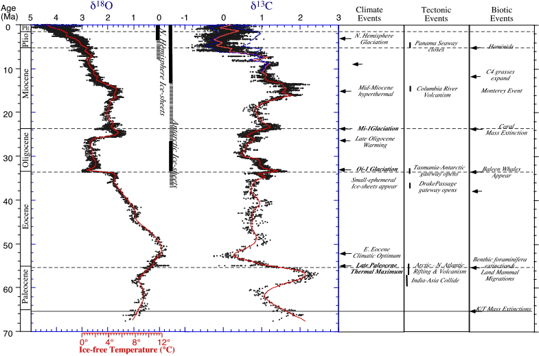
The Cenozoic record (see figure 2, below) clearly shows the following features, which have been recognized at many different sites in the world's oceans and thus can be seen as the record of global changes. During the Cenozoic the d¹⁸O values of benthic and planktonic foraminifera at high latitudes, and benthic foraminifera at low latitudes, increased, but the values in surface-water planktonic foraminifera at low latitudes showed little to no change. The increases did not occur gradually, but in "steps", intervals of sudden change, alternated with stable intervals. Major steps each lasted about 10⁵ years (one hundred thousand years) or less, and occurred in the earliest Oligocene (about 35.5 Ma; establishment of the east Antarctic ice sheet), the middle Miocene (13.6 Ma; increase in volume of the Antarctic ice sheet, possibly establishment of the west Antarctic ice sheet and small northern hemispheric ice sheets), and in the Pliocene (about 2.7 Ma, initiation of large-scale northern hemispheric ice sheets).

Figure 2. Oxygen isotope values (left column) for the Cenozoic, after Zachos, J., Pagani, M., Sloan, L., Thomas, E., and Billups, K., 2001, Trends, Rhythms, and Aberrations in Global Climate Change 65 Ma to Present. Science, 292: 686-693. Note that lower (more negative) d¹⁸O values mean that water temperature was higher, or the polar ice sheets were smaller, or both at the same time. Note temperature scale (given for ice-free conditions) below; see description of events to the right.